Summary:
You can raise the performance of your DAX code by applying filters in a sequential order from the most selective to least selective. The goal is to minimize the size of the data caches retrieved by the Vertipaq storage engine ‘up front’ thus rendering subsequent scans/queries faster as they operate on smaller data.
DAX Example: FILTER()
Brief background:
Filter(MSDN) is a table function that iterates the rows of the table or table expression you pass to it returning a TRUE() or FALSE() condition. The table returned by FILTER() is most commonly used as a filter to a CALCULATE() function or as a table to other functions like COUNTROWS() or SUMX. As FILTER() supports measure expressions and multiple AND() and OR() conditions it’s very powerful but for performance it has to applied with great care.
The requirement:
“Internet Sales for customers with both income of greater than $130K and sales of over $100.”
So we have two conditions that the customer table must respect – one that is very selective (309 customers out of 18,484 with $130K+ salaries) and one that is not selective at all (10,808 customers have over $100 in sales).
Two design approaches to building this metric:
The naïve approach:
CALCULATE
(
[Internet Sales $],
FILTER(Customer,AND([Internet Sales $]>100,Customer[YearlyIncome]>130000))
)
As mentioned you can do add many AND/OR clauses to a single FILTER function and for low granularity tables being iterated this might not be an issue. It may also make the code more readable than the superior approach:
The ‘think columnar’ approach:
CALCULATE
(
[Internet Sales $],
FILTER(
FILTER(Customer,Customer[YearlyIncome]>130000),
[Internet Sales $]>100)
)
With this approach, the designer ‘forces’ the storage engine to compute the YearlyIncome condition first in a separate scan. So when the Internet Sales condition is applied, it’s only applied on a tiny
*Note also that Internet Sales is a metric representing a SUM of the fact table whereas YearlyIncome is an attribute of the dimension with about 15 distinct values. So we’re scanning a very, very small amount of memory up front.
And the results (on this tiny, AdventureWorks data set):
30%+ faster via Think Columnar method
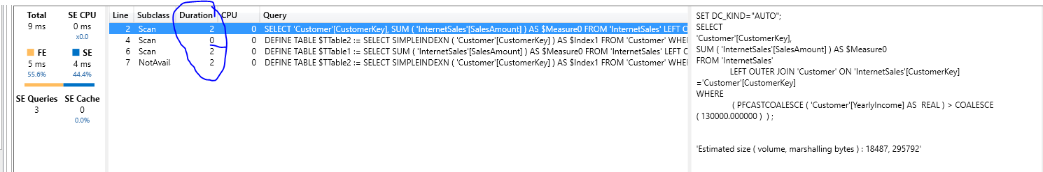
- Note that the first scan included the 130K filter with the Sales to Customer join. (Can see this in the right text box of image)
- Note that the second scan, which applied the second filter for $100 in sales or more, didn’t even register any MS for Duration. (We pitched a shutout! 🙂
Contrast this with the Naïve approach to FILTER:

For the NAIVE approach, the first scan is nothing more than a sum of sales with the join to Customer, no additional filter. The second scan takes 3MS because it’s operating on a larger data cache to apply both.
Takeaways:
Always be thinking of an efficient method for traversing between your larger dimensions (e.g. Product, Customer) and your fact tables. Look for an opportunity to cut down the granularity of one of these tables at query time before the values are passed over to the fact table. Be sure to use the most selective condition first, one column at a time.
A closely related point that I mentioned in Part I regarding RANKX is that the business may be completely ‘OK’ with faster yet specialized metrics. For example if you know there are many dimension members such as one-time customer purchases or expired products that, though clearly necessary in some general contexts they may not be needed for certain reports or dashboards. The purpose of many modern visual and interactive ‘experiences’ is not to tie to the GL but rather get a clear directional sense and thus in a columnar database with cardinality being the enemy of performance a query time filter on a high cardinality dimension may be a reasonable option to support performance and usability.
